
Create a Sensitivity Analysis Run
To access this screen:
-
Activate a sensitivity analysis case in the Project Map, then in the Tasks Pane choose Sensitivity Analysis >> Settings.
It is useful to understand how changes to schedule inputs affect the optimization workflow.
Understanding the risks and opportunities of your project is key, and by analysing your strategic plan's sensitivity to optimization parameters you can make more informed decisions about how your schedule and the intermediate data stages should be calculated.
Studio NPVS lets you set up a batch run of scenarios to compare outcomes where changes are made to key scheduling parameters including financial influences such as commodity price, mining cost, processing cost and recovery cost. Your optimization results will also be sensitive, potentially, to geophysical constraints such as slope angles and changes in stockpiled materials, for example.
Setting up a batch run is straightforward; first, define a base case with all parameter settings. Then, for each sensitivity analysis, define alternative values for one or more parameters.
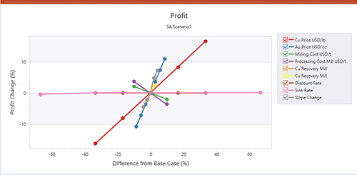
An example of a Sensitivity Analysis chart showing results for profit
For example, a base case is defined that describes the initial run's default parameters, such as product price, mining cost, sink rate, slope range and so on. In the base case, the copper price ($/lb) is 4.0. The schedule is then solved to provide the optimal extraction sequence based on this commodity price in conjunction with the other scheduling parameters (financial, physical, operational etc.). You want to see the impact on the schedule should copper fall to 3.0, so a sensitivity run is defined with only the commodity price altered.
You can then compare the tabular results via a summary report indicating comparative revenues, cost, NPV, ore and waste fractions and strip ratio for each sensitivity scenario. Results can be viewed graphically too, using the Group Chart function that presents useful spider charts highlighting the impact of setting changes on other elements of the schedule.
A sensitivity analysis scenario determines how the variation in an input variable (such as commodity prices, slope angle and so on) affects your output schedule and results. The differential output from each run can highlight how sensitive your case study is to a particular variable, allowing you to potentially make more risk-averse decisions when manipulating your optimization run settings.
Note: Sensitivity analysis settings are only accessible if the currently active scenario is of the expected type (a case study created from a base study using the Project Map's context menu). By default, these scenarios start with "Sensitivity...".
Screen Layout
The Define Custom Variables for Sensitivity Analysis Runs screen is used to define the nature of your batch run and, specifically, which variable(s) alter between runs. One or more variables can be adjusted.
It's a tabular view, with all customizable run variables listed vertically on the left (these can be filtered to show only particular variable types) and a series of table columns running from left to right; these represent the "Base Case" for your run, that is, the original scenario settings for economic model and ultimate pit from which the sensitivity analysis scenario was closed, followed by additional column entries where you wish to modify one or more attribute values.
For example, you may wish to assess the impact of a commodity price change on your optimization run results. In this case, the base case shows all attribute values in the leftmost column and you specify a new scenario name and commodity price value in the next column along:
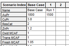
In the above example, the base commodity price for Gold is 1800, but a second run is added with identical settings other than a reduced (1500) gold price.
Tip: Changing multiple variable values for a sensitivity 'run', whilst supported, may make it difficult to assess how results are impacted by a single attribute change. However, cumulatively adding variables in subsequent runs may be informative; for example, changing the commodity price in sensitivity run 1, then changing a cost adjustment factor in run 2 produces two sets of results, but the impact of each variable change should be clear.
The list of adjustable variables for complex projects may get quite long, so consider using the filter options on the right to show more or fewer options. For example, you don't have to show mining cost adjustment factors (MCAFs) for each rock type of your scenario, or anything related to ultimate pit generation.
Once you've defined a batch run to test variable sensitivity, consider saving the settings to an external file. This could be useful, say, if you want to assess the same variable sensitivities for another base scenario or project, or to set up an organization standard run for all strategic planning projects prior to schedule approval or publishing.
Note: When sensitivity runs are processed, only scenarios with new data are processed. Previously completed scenarios are not run again if variable values are not changed.
Sensitivity Chart Results
Completion of a sensitivity run lets you compare the results of batch runs against key performance indicators for your project. Once a run is complete, chart creation (Optimization ribbon >> Charts >> New Chart) involves, as a first step, defining the number of KPIs to display using the Select Spider Graph KPIs screen.
Each selected KPI causes a new chart to be created within the Reports view. Charts can be shown either in independent or grouped viewing mode.
Within each chart, an axis plotted for each variable value change throughout the batch run. For example, a run testing the sensitivity of processing cost to commodity price, discount rate and per-bench MCAF could look like this:
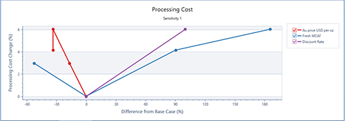
In the above example the processing cost % change is represented by the Y axis and the overall difference of the variable value from the base case (also a percentage) is represented by the X axis. In this example, the blue line (representing per-bench MCAF values) varies between 2.5% and 6% from the base case with the test values provided. Only one batch run included a change in discount rat, so only 2 values are shown as a straight line, whereas the commodity (AU) price and MCAF values were adjusted for all 3 non-base cases.
Activity Steps:
- Change your Project Default Settings to set the amount of system resources to be used during sensitivity analysis runs. This is adjusted using the Batch run options.
- Complete a base case scenario for at least one case, including at least economic model and ultimate pit settings. This is the scenario that will be varied in subsequent runs to assess sensitivity to variable changes.
- Display the Project Map control bar and select your base case (right click >> Case Study >> Select).
-
Right-click the base case again and choose Sensitivity Analysis.
A new case study appears in the Project Map called "Sensitivity" followed by an index number, e.g. "Sensitivity 3".
-
Right click the new sensitivity study and choose Case Study >> Select.
The case study shows in bold text.
- If needed, right click the sensitivity case and choose Case Study >> Rename.
- Save your project.
- Display the Task Pane and ensure the Optimization view is displayed.
-
Expand the Sensitivity Analysis menu item:
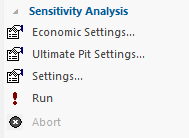
- By default, economic model and ultimate pit settings for your batch run will be the same as the original base case, although you can change these settings (which won't affect the base case) using the Economic Settings and Ultimate Pit Settings screens. See What is an Economic Model? and What Are Pit Shells?.
-
Select Settings.
The Define Custom Variables for Sensitivity Analysis Runs screen displays.
-
If you plan to use previously generated sensitivity run settings, already saved to a file, Load them and skip to this step.
-
Review the variables displayed vertically on the left of the table. By default, all customizable variables are shown.
-
Uncheck Show custom variables to remove any non-default optimization workflow variables from the list, such as those created using the Define Custom Variables screen.
-
Uncheck Show MCAF by rock type to remove all mining cost adjustment factor variables (for each defined rock type) from the table.
-
Uncheck Show MCAF by bench to remove per-bench mining cost adjustment factor variables from view.
-
Uncheck Show ultimate pit variables if you're not interesting in testing the sensitivity of variables used to establish the ultimate pit.
-
-
Change the Reference slope angle (for all sensitivity runs) if the current value isn't appropriate.
-
If you intend to reuse your sensitivity run settings again, Save them.
-
Review your settings and click OK to dismiss the Define Custom Variables for Sensitivity Analysis Runs screen.
-
Using the Task Pane, choose Sensitivity Analysis >> Run.
Economic model and ultimate pit data are generated wherever a new sensitivity scenario is detected. If this is the first time you have run sensitivity analysis for your project, all non-base cases are processed. Progress updates appear in the Batch Run Log window during processing.
On completion of the sensitivity analysis run, a default chart displays.
To review the results of the sensitivity analysis run and view more charts:
-
Once all runs are complete, activate the Summaries window and display the Sensitivity Analysis table. This displays a summary of all values used for all sensitivity scenarios and, further to the right, values for the following key optimization results:
-
Revenue
-
Processing Cost
-
Mining Cost
-
Rock tonnage
-
Total Ore
-
Total Waste
-
Strip Ratio
-
-
Create one or more spider graphs to see how variable changes affect key optimization performance indicators (KPIs) using Optimization ribbon >> Charts >> New Chart.
-
Choose which KPI(s) to show as an independent spider graph using the Select Spider Graph KPIs screen and click OK.
If custom report variables have been defined, they also appear here and can be represented as spider graphs.
-
Click Optimization ribbon >> Show >> Reports to display a spider graph for each selected KPI.
By default, spider graphs are shown in independent mode (one graph on view at a time, multiple tabs at the bottom of the screen) although you can display graphs concurrently using group chart mode. See Grouped Charts and Reports.
For example, all KPI charts selected for a run and all charts shown using grouped mode:
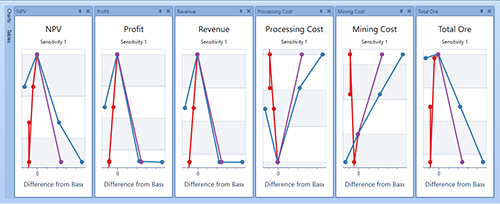
-
Hover the cursor over independent data points on a graph to see the values contributing to each plot point.
-
Save your project.
Related topics and activities